Orcad pspice designer

Как пользоваться программой LTspice/SwitcherCAD

Перейдем непосредственно к инструкции использования программы и как создать свою первую схему, после установки данного ПО на свой компьютер.

Создание нового файла

После запуска программы нас встретит стартовое окно (рис. 3). Для создания новой схемы необходимо в верхней части панели инструментов кликнуть на иконку 

FileNew SchematicDraftFileSave As

Рис. 3. Стартовое окно LTSpice.

Как только мы создали новый файл, на панели команд появились новые меню: Edit, Hierarchy, Simulate и Window, и рабочее поле редактора поменяло цвет на серый (рис. 4). При нажатии комбинации клавиш «Ctrl+G» или команд View (Вид) => Show Grid (Показать сетку) появится сетка на рабочем поле.

Рис. 4. Скриншот создания нового файла в LTSpice.

Полный список компонентов

В правой части панели инструментов можно найти часто используемые компоненты, такие как:

• резистор ;
•  конденсатор ;
• индуктивность ;
• диод ;

Для открытия полного списка компонентов можно выполнить одно из следующих действий: кликнуть на иконку 

EditComponentSelect Component SymbolOK рис. 5

Рис. 5. Выбор компонента из диалогового окна Select Component Symbol.

Как зеркально отобразить элемент в LTspice

При необходимости повернуть или зеркально отобразить компонент на рабочем поле применяется сочетание клавиш «Ctrl+R» или нажатие иконки 

• удаление одного и более элементов (вызывается клавишей F5 или нажатием на иконку );
• копирование одного и более элементов (вызывается клавишей F6 или нажатием на иконку );
• поиск элемента в схеме (нажатие на иконку );
• перемещение одного и более элементов (вызывается клавишей F7 или нажатием на иконку );
• перетаскивание одного и более элементов, отличается от предыдущего тем, что перетаскивает элемент или группу элементов без разрыва цепи (вызывается клавишей F8 или нажатием на иконку );
• возврат к прошлому состоянию (вызывается клавишей F9 или нажатием на иконку );
• возврат к последующему состоянию (вызывается сочетанием клавиш «Shift + F9» или нажатием на иконку ).

Так же, на схеме обязательно должен быть элемент «Земля» , с которым будут связаны все элементы вашей схемы, иначе программа не даст смоделировать процесс. Для того, чтобы связать все элементы цепи, вам необходимо нажать на иконку карандаша  или же через команду Edit (Редактирование) на панели управления.

Далее разберём какие анализы можно проводить в программе LTSpice.

PSpice simulation using each of the Relay’s Model

Following is an example of using each of the relay model for PSpice simulation: 

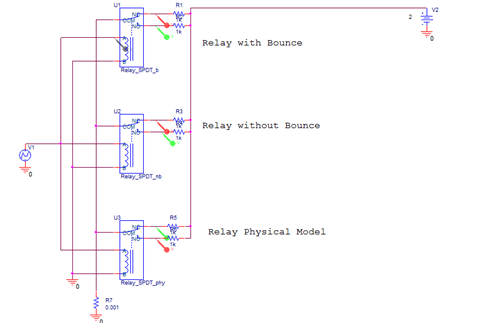
                        Figure 1: Relay Model Circuit

Figure 2 shows the results of the PSpice simulation of the Relay Model circuit.

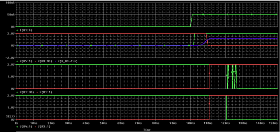
                                Figure 2: Output from Relay Model Circuit

Figure 2 shows a Probe plot of the input current, and the output voltages of each of the relay model from each circuit.

Note: Circuits with physical relay model may take longer time to simulate in comparison to circuits without physical model.

Copyright 2016 Cadence Design Systems, Inc. All rights reserved. Cadence, the Cadence logo, and Spectre are registered trademarks of Cadence Design Systems, Inc. All others are properties of their respective holders.

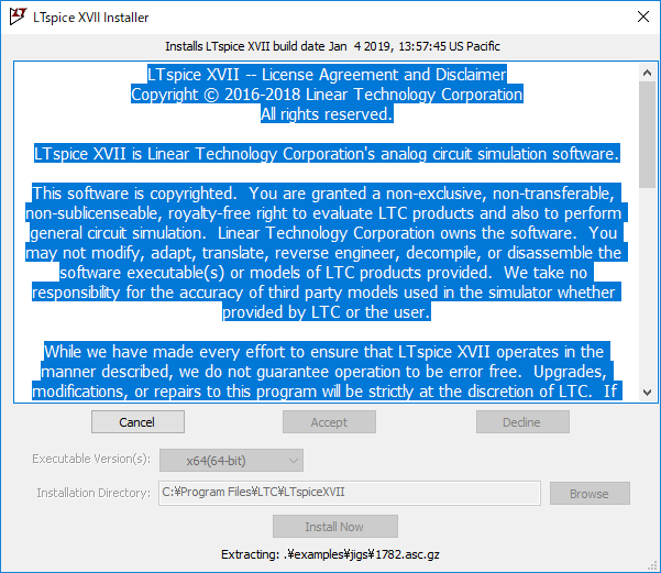
Install LTspice XVII

Launch the installer by double-clicking the downloaded executable file (exe file).

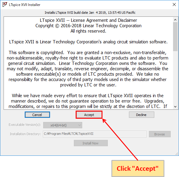
Click “Accept”.

Click “Install Now”

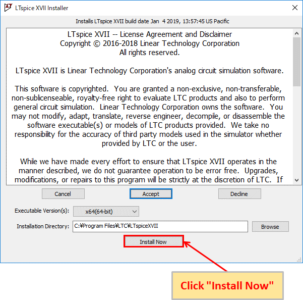
You can select 64bit or 32bit in “Executable version (s)” and the folder to install in “Installation Directory”. If nothing is wrong, click Install Now.

The installation will start, so wait for a while.

Click “OK” when the installation is successful

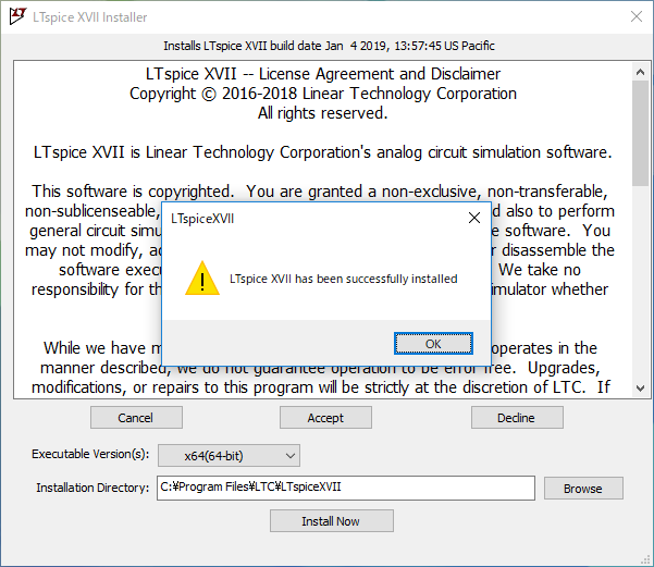
If the message “LTspice XVII has been successfully installed” is displayed, the installation has been successfully completed. click “OK”.

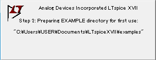
Since LTspice XVII starts up automatically, wait for a while if there is the above display.

Automatic startup and shortcut icon generation for LTspice XVII

Finally, LTspice XVII starts up. You should have a shortcut icon on your PC desktop.

This completes the download and installation method of LTspice XVII.

DipTrace скачать бесплатно через торрент, по прямой ссылке с русификатором

DipTrace 3.3 Trial — пробная «trial» версия на 30 дней, включены все функции и библиотеки (без 3D моделей).

DipTrace 3.3 Freeware — бесплатная версия, включены все функции и библиотеки (без 3D моделей), ограничение на 300 выводов и 2 сигнальных слоя.

DipTrace 3.3 Mac — бесплатная для некоммерческого пользования, доступны все функции и библиотеки (включая 3D модели), ограничение на 300 выводов и 2 сигнальных слоя. Перед установкой DipTrace на Mac OS X требуется установить XQuartz X11.

После скачивания файла, его необходимо установить в папку с установленной программой DipTrace.

При необходимости вернуть интерфейс к английскому языку, достаточно удалить всей файлы с расширением *.lng из папки «C:\ProgramData\DipTrace\Data».

How to convert SPICE Netlist to an LTspice schematic

Schematic Builder to automate the first steps below.

Before you start, make working copy of the netlist and then clean
it up by doing any reordering of lines or shortening of node/net
names that will make them easier to work with. For example, nets
with names like «n023» and «n001» can usually be safely shortened
to «n23» and «n1» (sometimes I do this in a word processor with
find and replace). Also, it is a good idea to move all comments
to the end of the working netlist (if not delete them altogether).

At this point, I like to import the netlist into LTspice, either
directly onto the schematic (if the netlist is short) or into a
separate LTspice netlist window.

Now go through the netlist line by line and place a component of
the corresponding type on the schematic (arrange these in rows by
component type such that you build up rows of all the same type).
It is important to do this in exactly the same order as the net-
list because this will greatly ease cross checking when you think
you have finished. (Also, all of the SPICE text, such as model
statements, etc. should be copied and pasted in at the end.)

As you place each component, edit its reference designator to
agree with the corresponding netlist reference designator.

As you place each component, place a net-label/node-name directly
on each pin of the component (of course, these should agree with
their names in the netlist, too). Don’t bother with wires yet as
these will just be trouble to move around later.

Once all the components are placed, view the SPICE Netlist (it’s
a drop-down menu item) and verify that it agrees *exactly* with
the original netlist (it will, if you followed these instructions
carefully). Correct any errors as needed until agreement is
perfect. This «schematic» should actually be able to run at
this point.

(This above section is what is automated by the SchBuilder.)

So far you have just been playing the part of a robot, but now
comes the fun part where human judgement is required. Move the
components around on the schematic to group them such that the
pins that have the same net names are close to each other and
that signal flow makes sense. Use the Highlight Net tool (right
mouse button click on a pin or net) to make sure no connection
is overlooked.

Only when the parts are reasonably well placed is it time to
start drawing in the wires and adjust the look of the schematic.

Be sure to check occasionally that the two netlists continue to
match.

Because both netlists and schematics are just ascii text files,
the first part of this process should be fairly straightforward
to automate in software. Grouping components and connecting them
for least total wire length might be harder, but still possible
(I would try an approach using the so-called «synthetic annealing»
algorithm). However, finishing the schematic to human sensibilities
would seem beyond the reach of any canned program, but having a
utility that did the first two steps would be a big time saver and
well worthwhile. (from analogspiceman, used by permission)

Source Code for Schematic Builder is available here or
as one zip file available here
You need to use Lazarus a Pascal based development tool.
After you have installed the latest version of Lazarus, double-click on SchBuilder.lpr to open the project. Further development and LTwiki updates are encouraged.

waveform delete

You can delete the waveform with the “Expression Editor” or “Cut” on the toolbar.

Expression Editor

1

When you move the cursor to the node name on the graph pane, the cursor changes to a finger mark, so right click of mouse.

This time, let’s delete the power waveform of “V(OUTPUT)*I(R2)”, so I do a “right click” of the mouse with the node name of “V(OUTPUT)*I(R2)”.

2

The “Expression Editor” will appear. Click “Delete this Trace”.

3

If you check the graph pane, you can see that the power waveform of “V(OUTPUT)*I(R2)” has been deleted.

Cut

1

Activate the graph pane and click “Cut” on the toolbar.
(It is OK to activate the graph pane and click “Plot Settings”-“Delete Traces” on the menu bar.)

After that, move the scissors mark(cursor) to the node name you want to delete and “left click” of the mouse.

This time, delete the power waveform of “V(OUTPUT)*I(R2)”, so “left click” of the mouse with the node name of “V(OUTPUT)*I(R2).

2

If you check the graph pane, you can see that the power waveform of “V(OUTPUT)*I(R2) has been deleted.

Waveform scaling

You can zoom in / out the waveform by setting commands on the toolbar or setting the scale of the graph.

Zoom to Rectangle

1

Activate the graph pane, click “Zoom to rectangle”, and while holding down the left mouse button, specify the area you want to enlarge.
(It is OK to activate the graph pane and click “View”-“Zoom Area” on the menu bar.)

2

The specified range is expanded as shown above.

Pan

1

Activate the graph pane, click “Pan”, and click the place you want to use as the reference of the display.
(It is OK to activate the graph pane and click “View”-“Pan” on the menu bar.)

2

As shown above, the point clicked with the mouse is the center of the vertical axis(Y-axis).

Zoom back

1

Activate the graph pane and click “Zoom back”.
(It is OK to activate the graph pane and click “View”-“Zoom back” on the menu bar.)

2

The waveform is reduced as shown above.

Zoom to extents

1

Activate the graph pane and click “Zoom to extents”.
(It is OK to activate the graph pane and click “View”-“Zoom to Fit” on the menu bar.)

2

The entire waveform will be displayed as shown above.

Vertical Axis(Y-Axis)

1

When you move the cursor to the vertical axis(Y-axis), the cursor changes to a ruler, so you can right click of the mouse.

2

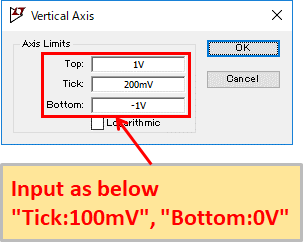
The “Vertical Axis” screen appears, so you can set the vertical axis(Y-axis) scale arbitrarily.

This time, let’s try to input “Tick: 100mV”, “Bottom: 0V”.

Vertical Axis Setting

• Top：Maximum value of scale
• Tick：Interval value of scale
• Bottom：Minimum value of scale

3

Click “OK” after entering.

4

As shown above, the vertical axis scale changes, and the waveform display changes to match the scale.

Horizontal Axis(X-Axis)

1

When you move the cursor to the horizontal axis(X-axis), the cursor changes to a ruler, so you can right click of the mouse.

2

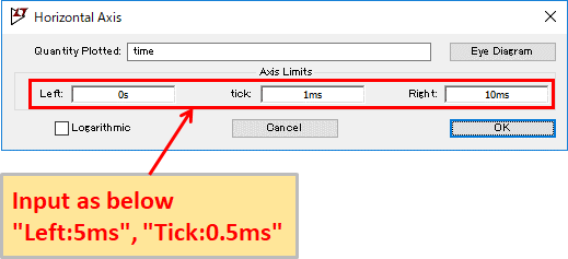
Since the “Horizontal Axis” screen appears, you can set the scale of horizontal axis(X-axis) arbitrarily.

This time, let’s try to input “Left: 5ms” and “Tick: 0.5ms”.

Horizontal Axis Setting

• Left：Minimum value of scale
• Tick：Interval value of scale
• Right：Maximum value of scale

3

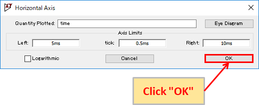
Click “OK” after entering.

4

As shown above, the scale of the horizontal axis is changed, and the waveform display changes according to the scale.

Примеры

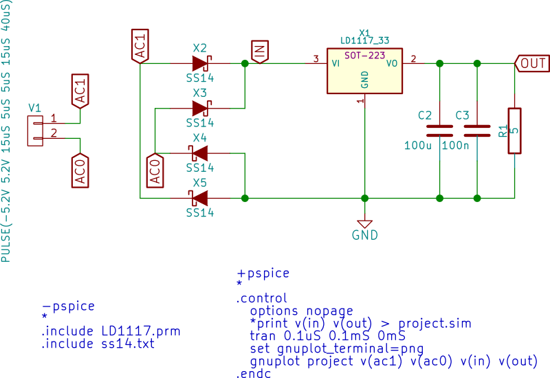
Дабы развеять туман в голове, давайте уже что-нибудь попробуем симулировать. Для начала что-то простое, я взял выпрямитель и линейный регулятор.

Схема абсолютно тупая, ибо наша цель её проанализировать. Конечно, я был несколько ленив и неаккратен, ибо не использовал общепринятые условные графические обозначения например для источника пульсирующего напряжения. Но это всё на результат не влияет, так что прошу меня извинить.

Здесь я разместил текстовые блоки, которые начинаются с —pspice и +pspice. В этих блоках расположены команды, которые будут вставлены до и после списка цепей соответственно. До списка цепей я добавил команды подключения (.include) файлов описания компонентов LD1117 и ss14. Это что-то вроде библиотек.

А после списка цепей я добавил блок .control, который описывает, что собственно мы хотим добиться от симулятора. Вот что делает каждая строчка:

.control * открываем блок
  * отключаем разбивку выводимых данных на страницы
  options nopage
  * вывод значений напряжения в точках in и out я временно закомментил
  *print v(in) v(out) > project.sim
  * симуляция переходных процессов с шагом в 1 микросекунду на интервале до 1 миллисекунды с началом в 0 миллисекунд
  tran 1uS 1mS 0mS
  * переключил вывод в png, чтобы потом вставить полученную картинку в этот блог
  set gnuplot_terminal=png
  * используем gnuplot для вывод графиков напряжений в точках ac1, in и out
  gnuplot project v(ac1) v(in) v(out)
.endc * закрываем блок

Это в принципе всё, что нам нужно, чтобы начать симуляцию. В EEschema надо при экспорте списка цепей выбрать экспорт в spice:

На выходе у меня получился файл project.cir вот с таким содержимым:

* EESchema Netlist Version 1.1 (Spice format) creation date: Вт 10 мар 2015 22:00:26

* To exclude a component from the Spice Netlist add  user FIELD set to: N
* To reorder the component spice node sequence add  user FIELD and define sequence: 2,1,0
.include LD1117.prm
.include ss14.txt

*Sheet Name:/
R1  OUT GND 10		
X1  GND OUT IN LD1117_33		
V1  AC1 GND PULSE(-2.7V 2.7V 0 5uS 5uS 15uS 40uS)		
C1  IN GND 470u		
C2  OUT GND 100u		
X2  AC1 IN SS14		
C3  OUT GND 100n		

.control
  options nopage
  *print v(in) v(out) > project.sim
  tran 1uS 1mS 0mS
  set gnuplot_terminal=png
  gnuplot project v(ac1) v(in) v(out)
.endc

.end

В качестве источника питания я использовал генератор прямоугольных импульсов. Это примерно соответствует вторичной обмотке трансформаторов импульсных блоков питания. Вот как он определён в ngspice:

PULSE (напряжение нуля, напряжение импульса, начальная задержка, время нарастания, время спада, длительность импульса, период импульсов)

В нагрузку я просто поставил резистор на 10 Ом, что-бы получить примерно 1 Ватт мощности на 3.3 Вольтах (3.3^2/10).

Мы можем получить значения напряжений и токов в точках функциями v(имя цепи) и i(имя цепи) соответственно. Кроме того, чтобы получить разность потенциалов между двумя цепями можно указать два значения в функции, например v(одна цепь, другая цепь). Можно даже производить вычисления.

Теперь осталось запустить симулятор командой: ngspice -b project.cir (просим его выполнить команды в фоновом режиме). Естественно у нас должны быть все подключенные файлы модулей. На просторах сети я нашел диод шоттки SS14 и библиотеку линейных регуляторов LD1117 от серьёзных вендоров, которым можно доверять.

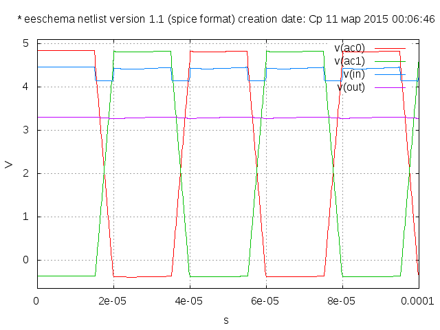
Вот какой график я получил:

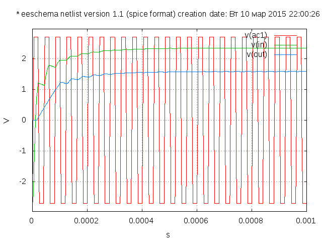
Забавно? Я тоже так думаю ^_^

Давайте не отходя от кассы поэкспериментируем, редактируя параметры прямо в полученном project.cir. Мы хотели бы получить на выходе как минимум 3.3V, а из результата симуляции сразу видно, что входного напряжения недостаточно. Зададим амплитуду 5.2V вместо 2.7V и повторим симуляцию:

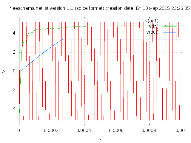
Теперь совсем другое дело.

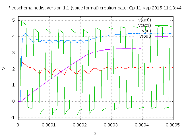
А теперь давайте немного изменим схему:

Я заменил диод мостом и убрал входную ёмкость. Также увеличил нагрузку до 2 Ватт. Затем увеличил масштаб времени симуляции, и добавил график напряжения в точке ac0.

Вот что получилось:

А теперь давайте попробуем по-другому. Предположим, что трансформатор выдаёт импульсы амплитудой всё те же 2.5V, то есть на одном выводе относительно другого имеем импльсы +2.5V и -2.5V. Изменим конструкцию выпрямителя так, чтобы получить 5V, использовав два диода и два конденсатора:

Повторим симуляцию, и посмотрим графики:

Как видим, получили именно то, что было нужно. А теперь посмотрим на графики напряжений относительно точки AC0:

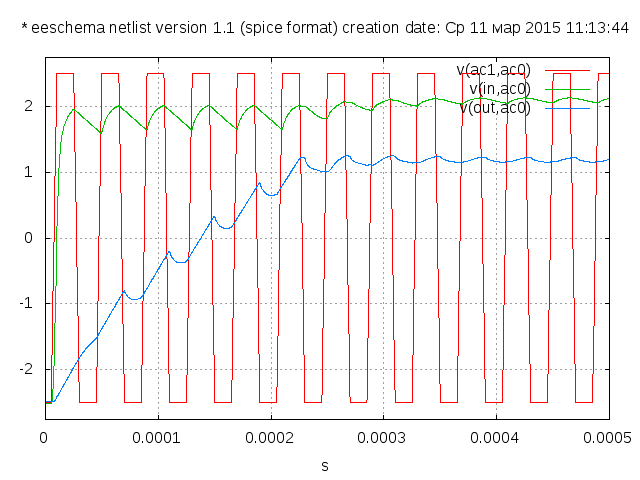
Исходники искать в репозитории: bitbucket.org:kayo/voltage_regulator, каждый вариант схемы в отдельной ветке.

На этом пока закончим. В следующий раз симулируем более интересную схему — детектор нуля сетевого напряжения с гальванической развязкой.

Comparing LTspice and Oscilloscope Waveforms

Sometimes you want to see how closely your SPICE simulation matches the real circuit as seen by your scope. Here is a utility which imports an LTspice waveform and the data from your scope, overlays them, and allows you to slide one back and forth to line them up. It’s called CompareWaveforms, and here’s what it looks like:

You select the files to compare, press Compare, and use the long slider along the bottom to line up the waveforms. You can save the plot as a .png file to include in a report.

The formats of the input files are straightforward. The LTspice file is the direct output of File / Export from the LTspice waveform window. The scope file is a .csv (Comma-Separated Values text file) with two header lines at the beginning (because that’s what my scope puts out). Each subsequent line is of the form time-in-seconds, volts. These are easily changed in the Python source if you wish. The scope data file may have a time offset due to trigger delay or trace positioning, so that is subtracted from the scope time measurements to match the LTspice time which starts at zero.

Note on waveform comparison: you may want to include the loading of your scope probe in your simulation. My probes are 12 pF in parallel with 2.2 Mohm, which can alter the simulator waveforms. Also, make your total simulation time equal to the sweep time of your scope (typically the time/div times 10), and make the start of the waveform roughly the same. CompareWaveforms allows you to adjust time +/-10% of the total sweep.

Описание и возможности LTspice (SwitcherCAD)

Программа LTspice является инструментом для всестороннего анализа электрических и электронных схем. В статье не рассматриваются вопросы, связанные с теорией, используемой для моделирования реальных систем, мы сосредоточимся только на результатах, полученных от пользователя, которому не нужно знать все эти теории.

Программа LTspice предоставляет помимо стандартного набора, ряд дополнительных инструментов, которые помогут вам вывести схемы и выбрать варианты моделирования, а также окончательную презентацию результатов. Некоторые из них активны только в коммерческой версии программы, но их блокировка лишь немного ограничивает функциональность программы.

Программа имеет очень простой и интуитивно понятный редактор. Вам не нужно знать язык Spice для моделирования, хотя в некоторых случаях это может облегчить вашу работу. Каждая симуляция начинается с построения схемы. Для этого используется встроенный графический редактор. Пользователь с помощью мыши и команд, содержащимися в меню или запускаемыми с помощью сочетаний клавиш, выбирает элементы из библиотек, встроенных в программу, и объединяет их, создавая принципиальную схему (рис. 1). Для каждого элемента назначаются поля, описывающие схематическое обозначение и номинальное значение (сопротивление, ёмкость, тип интегральной схемы, тип диода и т. д.).

Рис. 1. Схематично смоделированная система, созданная во встроенном редакторе программы LTSpice.

The Electrical(Behavioral) Model Approach

The second and third approaches simply model the electrical behavior of the relay coil and contacts. Rather than requiring physical construction parameters, these models require behavioral parameters.

Model of a Relay(without Contact Bounce)

The first behavioral model does not include contact bounce, and is the fastest to simulate. It requires parameters for coil inductance and resistance, contact resistance, pull-in and dropout coil currents, and make and break times. The model uses a PSpice digital buffer’s propagation time to model the make and break times, and uses the Analog to Digital conversion device to model the pull-in/dropout current hysteresis. It uses a Digital to Analog conversion device in an unusual configuration to model the contacts. By using the digital devices, it is easy to set the delays using sub-circuit parameters, and there are no time step problems that can be caused by very high gain analog switches. The following circuit file shows the simple behavioral model of a relay (without contact bounce). 

Model of a Relay(with Contact Bounce)

In some systems the previous model is too simple, since it does not include contact bounce. This model includes contact bounce for a specified period of time after the contacts close. The contact bounce is created by taking a digital contact close signal and converting it to an analog ramp using a Digital to Analog conversion device. The analog ramp forms the input to a table-controlled voltage source. The table creates a bounce output voltage which is then converted to digital to square it up. The digital value is used to control another Digital to Analog conversion device which models the contacts.

Note: Contact bounce is caused by the physical bouncing of the electrical contacts as they close. It looks electrically as if the relay contacts close and open several times in quick succession before they remain closed.

Что можно проанализировать с помощью моделирования

Хотелось бы сказать все, но, конечно, это не так. Тем не менее, объем анализа включает все наиболее важные параметры каждой электрической цепи:

«Transient» — анализ переходных процессов, в результате которого исследуется поведение электрической цепи при подачи питания. Пользователь определяет время моделирования, опуская исходный фрагмент заданной длины, в котором могут возникать переходные процессы. Есть еще несколько вариантов выбора (рис. 6).

Рис. 6. Измерение отклика системы на вынужденный сигнал.

«AC Analysis» — анализ переменного тока или исследование частотной характеристики системы. Указывается тип развертки частоты (Octave, Decade, Linear, List), количество точек, начальная и конечная частота (рис. 7). На диаграммах показаны амплитудные и фазовые характеристики напряжения или тока в указанной точке схемы.

Рис. 7. Частотный анализ системы.

«DC sweep» — постоянная кривая переходного тока U wy = f (U in ). Параметры этого измерения: источник или источники входного сигнала и выходной узел, который обычно является выходом системы. В этом моделировании все конденсаторы открыты, а индуктивность закорочена (рис. 8).

Рис. 8. Анализ переходных характеристик.

«Noise» — шум. Анализ шума линеаризованной схемы для фиксированной рабочей точки постоянного тока. Параметры этого измерения: выходной узел, источник входного сигнала, тип развертки (Octave, Decade, Linear, List), количество точек, начальная и конечная частота (рис. 9). В результате моделирования получены характеристики шума как функции частоты.

Рис. 9. Анализ шума тестируемой системы.

«DC Transfer» — функция передачи постоянного тока для малых сигналов, приводящая к значению усиления, входному и выходному импедансу (рис. 10).

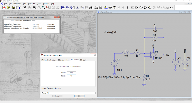
Рис. 10. Анализ «переноса постоянного тока».

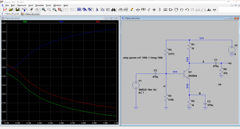
«DC op pnt» — постоянная рабочая точка. Напряжения рассчитываются во всех узлах тестируемой цепи и токов во всех ветвях (рис. 11). Информация об этих параметрах представлена в сводке в таблице. После наведения курсора на выбранный узел схемы, в нижнем углу экрана отображается информация о напряжении в этом узле, и после нажатия на это напряжение постоянно помещается на диаграмме. Чтобы получить информацию о ветвящихся токах аналогичным образом, необходимо сделать то же самое, указывая на элемент схемы в выбранной ветви. В дополнение к току дается мощность, рассеиваемая в этом элементе.

11(а).

11(b).

Рис. 11. Расчет постоянной текущей точки a) для значений фиксированного элемента, b) для значений параметрических элементов.

The Mechanical Model Approach

The mechanical model for the relay is modeling the mechanical part of electromechanical devices in general, using the relay as an example. This model constructs an electrical analogy to the mechanical operation of the relay. To do this, it calculates the magnetic and mechanical forces acting on the contact arm of the relay, and simulates the acceleration, velocity, and position of the arm in response to these forces. The electrical contacts of the relay are simulated by switches controlled by the position of the contact arm. There are two problems with this modeling approach: first it requires information about the physical construction of the relay (spring force, contact arm moment, magnetic permeance as a function of contact arm position) that is not normally available to the user of a relay, and second, it takes a lot of computer time to simulate the exact position of the contact arm. Most of this time is wasted if all the user needs to know is whether the contacts are open or closed. This type of physical model could be useful for designing a relay, but it is overkill for simulating its electrical behavior.

LTspice folder/file structure

Before going into the SPICE model, let’s first understand the folder and file structure of the latest version of LTspice XVII.

LTspice folder/file structure

• C:\Users\USER\Documents\LTspiceXVII
  • \examples: Stores example schematic file
  • \lib
    • \cmp: Store data file
      • \standard.res: Resistor
      • \standard.cap: Capacitor
      • \standard.ind: Inductor
      • \standard.bead: Ferrite bead
      • \standard.dio: Diode
      • \standard.bjt: Bipolar transistor
      • \standard.jft: J-FET
      • \standard.mos: MOS-FET
    • \sub: Store sub file and lib file
      • \*.sub: Sub file
      • \*.lib: Lib file
    • \sym: Store schematic symbol file

      \*.asy: Schematic symbol file

Especially the cmp folder, sub folder, sym folder and the files under it that make up the lib folder are important for understanding the SPICE model.

Changes in LTspice XVII

The changes from the old version LTspiceIV to the new version LTspiceXVII are as follows.

Changes from LTspice IV to LTspice XVII

• 64-bit compatible (simulation speedup)
• Character font supports Unicode (Japanese can be described in the schematic)
• GUI change (improves operability and usability)

etc.

As a major change, LTspiceXVII supports 64 bits, and according to the “LTspiceXVII Startup Guide”, simulation is 26% faster than previous versions of LTspiceIV.

In addition, because the character font corresponds to Unicode, it is possible to describe Japanese in the circuit diagram.

And the change in GUI has improved operability and usability compared to previous versions of LTspice IV.

Описание

DipTrace — это расширенный пакет инструментов для проектирования печатных плат, состоящий из 4 функциональных модулей:

• PCB Layout — основной редактор печатных плат с интегрированным двухмоторным автоматическим маршрутизатором и трехмерным предварительным просмотром;
• Schematic Capture — редактор схем;
• Component Editor — редактор символов, которые позволят расширить стандартную базу данных;
• Pattern Editor — редактор шаблонов.

DipTrace — очень простой редактор в обучении, интуитивно понятный интерфейс, а так же доступные обучающие материалы на веб-сайте, помогут пользователю шаг за шагом на всех этапах проектирования. Преобразование схемы в файл-макет PCB одним щелчком мыши, расширенные функции соединения компонентов и встроенный авто-трассировщик позволяет пользователю быстро завершить проект. Сравнение и обновление данных из схемы может быть выполнено на любом этапе проекта.

Программа также обеспечивает поддержку внешнего авторутера благодаря интерфейсу SPECCTRA, проверку правил соединения ERC и принципам проектирования DRC. Модули DipTrace позволяют обмениваться схематическими файлами, печатными схемами, библиотеками символов и чертежами цепей с другими пакетами EDA и CAD. Редактор схем также предлагает поддержку популярных форматов SPICE .CIR. Стандартом также являются производственные форматы для сверления и фотоплоттера Gerber, NC Drill, G-Code Mach 2/3.

ПО доступно для платформ: Windows XP / Vista / 7 / 8 / 8.1 / 10; Linux (Wine); Mac OS X (необходим XQuartz).

LTspice Induction Motor Simulation

I have been looking at existing simulation models for induction motors and found a particularly interesting one by Sohor and Kubov that appears several places on the Internet. I used the Spectrum Software application note about this model as a starting point and, after much pain, got a working induction motor model in LTspice. However, it turns out that a working version of this model had already been created for LTspice and uploaded to our group’s files section.

Going through the painful process of reinventing the wheel (or motor) was not all for naught because in doing so I got to understand how the model works. It actually is very compactly written to the point of obscuring its basic operation. I have deconstructed it into its various parts as separate function modules in order to facilitate understanding. The original SK model uses transformer coupling coefficients to implement the three phase to two phase (DQ) translation and to implicitly build the inductive T-network that represents the stator, air gap and rotor. This requires the use of negative and zero coupling coefficients, making it very difficult to understand how the model works. Also the SK model indirectly accesses flux by looking at current times inductance, which only works with ideal, linear inductances. I have separated these various functions and more directly modeled flux so that saturating inductance (LTspice’s Chan model) can be used in order to model motor saturation (assuming no mistakes have been made along the way).

When an induction motor first starts, the rotor is at a standstill and the sees the full line frequency, but as it speeds up, it sees only the difference between its angular speed and the stator field rotating at the line frequency, which may be a fraction of a Hertz at full speed. This frequency shift in the rotor’s frame of reference affects the penetration depth of rotor current and its effective resistance and inductance. The basic SK model does not address this effect at all, but it may be possible to add these effects to the LTspice version of the model. — a.s.

Model Here: File:Simplified 2-Phase Induction Motor (with saturation).ascMore Complete files including 3 phase motors

Дополнительные возможности

По сравнению с исходным проектом Spice3f5 NGSPICE получил возможность моделирования критических устройств в схеме, моделирования пользовательских нодов, отличных от тока, напряжения и логических уровней, а также симулирования аналоговых и цифровых цепей. Появилась возможность в дополнение к классическому интерфейсу командной строки использования графического интерфейса через язык TCL. Кроме того, были добавлены новые модели устройств, а также облегчена возможность добавления пользовательских аналоговых и цифровых моделей.

Cider

Симулятор на уровне устройств из проекта Cider обеспечивает дополнительные возможности для более точного моделирования схем с учетом моделирования критически важных элементов. Для моделирования элементов используются два симулятора: встроенный симулятор DCIM и интерфейс с внешним симулятором устройств GSS TCAD.

Встроенный симулятор DCIM использует язык описания устройств из проекта PISCES, разработанный Станфордским университетом, и классическое для SPICE описание схемы соединений.

XSPICE

NGSPICE использует комбинированный симулятор смешанных сигналов из проекта XSPICE. Фактически, он добавляет в симулятор цифровые ноды, характеризуемые логическим уровнем и мощностью сигнала.

Для добавления моделей цифровых устройств может использоваться либо написание модели на языке C либо использовать специально предусмотренный интерфейс для внедрения цифровых моделей, написанных на языке описания и моделирования аппаратуры Verilog

TCLSpice

Интерфейс позволяет написание графических оболочек для более тесного взаимодействия с симулятором с помощью команд на языке TCL