Модуляция
Содержание:
End-to-end simulation
The complete waveform simulation for the end-to-end transmission of information using BPSK modulation is given next. The simulation involves: generating random message bits, modulating them using BPSK modulation, addition of AWGN noise according to the chosen signal-to-noise ratio and demodulating the noisy signal using a coherent receiver. The topic of adding AWGN noise according to the chosen signal-to-noise ratio is discussed in section 4.1 in chapter 4. The resulting waveform plots are shown in the Figure 2.3. The performance simulation for the BPSK transmitter/receiver combination is also coded in the program shown next (see chapter 4 for more details on theoretical error rates). The resulting performance curves will be same as the ones obtained using the complex baseband equivalent simulation technique in Figure 4.4 of chapter 4.
Refer Digital Modulations using Matlab : Build Simulation Models from Scratch for full Matlab code.Refer Digital Modulations using Python for full Python code
File 3: bpsk_wfm_sim.m: Waveform simulation for BPSK modulation and demodulation
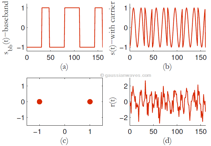
Figure 3: (a) Baseband BPSK signal,(b) transmitted BPSK signal – with carrier, (c) constellation at transmitter and (d) received signal with AWGN noise
Binary Phase Shift Keying (BPSK)
Binary Phase Shift Keying (BPSK) is a two phase modulation scheme, where the 0’s and 1’s in a binary message are represented by two different phase states in the carrier signal:
In digital modulation techniques, a set of basis functions are chosen for a particular modulation scheme. Generally, the basis functions are orthogonal to each other. Basis functions can be derived using Gram Schmidt orthogonalization procedure . Once the basis functions are chosen, any vector in the signal space can be represented as a linear combination of them. In BPSK, only one sinusoid is taken as the basis function. Modulation is achieved by varying the phase of the sinusoid depending on the message bits. Therefore, within a bit duration
|
This article is part of the following books |

where,
The constellation diagram for BPSK (Figure 3 below) will show two constellation points, lying entirely on the x axis (in-phase). It has no projection on the y axis (quadrature). This means that the BPSK modulated signal will have an in-phase component but no quadrature component. This is because it has only one basis function. It can be noted that the carrier phases are
Topics in this chapter
|
Digital Modulators and Demodulators — Passband Simulation Models ● Introduction ● Binary Phase Shift Keying (BPSK) □ BPSK transmitter □ BPSK receiver □ End-to-end simulation ● Coherent detection of Differentially Encoded BPSK (DEBPSK) ● Differential BPSK (D-BPSK) □ Sub-optimum receiver for DBPSK □ Optimum noncoherent receiver for DBPSK ● Quadrature Phase Shift Keying (QPSK) □ QPSK transmitter □ QPSK receiver □ Performance simulation over AWGN ● Offset QPSK (O-QPSK) ● π/p=4-DQPSK ● Continuous Phase Modulation (CPM) □ Motivation behind CPM □ Continuous Phase Frequency Shift Keying (CPFSK) modulation □ Minimum Shift Keying (MSK) ● Investigating phase transition properties ● Power Spectral Density (PSD) plots ● Gaussian Minimum Shift Keying (GMSK) □ Pre-modulation Gaussian Low Pass Filter □ Quadrature implementation of GMSK modulator □ GMSK spectra □ GMSK demodulator □ Performance ● Frequency Shift Keying (FSK) □ Binary-FSK (BFSK) □ Orthogonality condition for non-coherent BFSK detection □ Orthogonality condition for coherent BFSK □ Modulator □ Coherent Demodulator □ Non-coherent Demodulator □ Performance simulation □ Power spectral density |
OOK vs FSK vs ASK | Difference between OOK, FSK, ASK modulation
This page compares OOK vs FSK vs ASK and describes difference between OOK, FSK and ASK modulation techniques.
OOK Modulation | ON OFF Keying Modulation
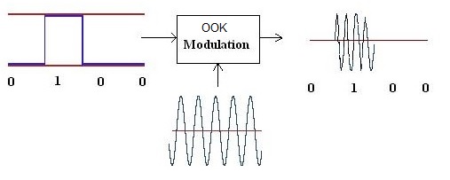
The figure-1 depicts OOK modulation technique.
OOK stands for On Off Keying. OOK is modified version of ASK modulation.
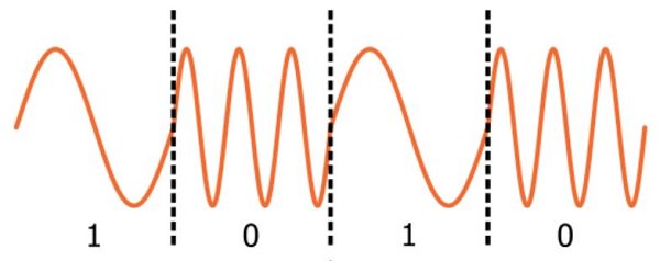
While in ASK modulation logic-0 is represented by lower amplitude and logic-1 is represented by higher amplitude;
in OOK modulation there is no carrier during the transmission of logic zero.
The carrier is transmitted during the transmission of logic one.
In OOK modulation transmitter goes to IDLE state during transmission of logic «zero».
This will help in conserving battery power.
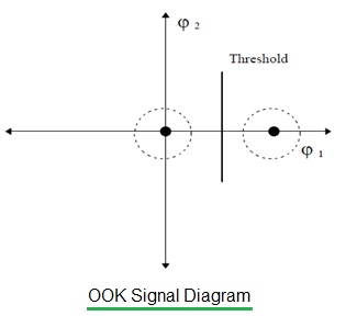
The figure-2 depicts OOK signal diagram. Here φ1 and φ2 represent signal vectors or complex data.
The additive noise is represented by dotted circle around the main signal points.
As shown one vector (φ1) represent some amplitude on X-axis while
the other vector (φ2) represent zero value.
As carrier wave is present and absent at two different logic states, this modulation type is known as ON OFF Keying or OOK modulation.
ASK Modulation | Amplitude Shift Keying Modulation
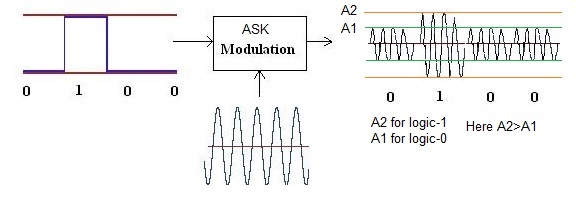
The figure-3 depicts ASK modulation and FSK modulation techniques.
ASK stands for Amplitude Shift Keying.
In ASK modulation, modulating input is digital and carrier is analog.
The carrier wave is present with higher amplitude(i.e. A2 as shown) in ASK modulated output where binary input
is ‘one’ is to be transmitted. The logic zero is transmitted with lower amplitude (i.e. A1) compare to logic-1.
Also Refer 10ASK and 100ASK modulation >> used in NFC technology.
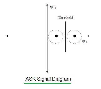
The figure-4 depicts ASK signal diagram. As shown one vector (φ1) represent
higher amplitude compare to the other vector (φ2).
The higher the difference between the two amplitudes, easier to detect and decode
the data signal points at the receiver.
As amplitude value is shifting in transition from one binary logic to the other, this modulation type is known as
amplitude shift keying.
FSK Modulation | Frequency Shift Keying Modulation
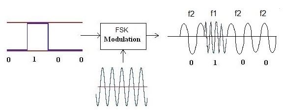
FSK stands for Frequency Shift keying.
In FSK modulation, modulating input is digital and carrier is analog.
Modulated output will have frequency of f1 when binary input is ‘one’ and
it will have frequency of f2 when binary input is ‘zero’.
Also refer 2FSK vs 4FSK modulation >>.
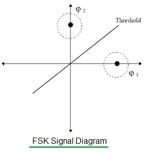
The figure-5 depicts FSK signal diagram. As shown one signal vector (φ1) is represented by some phase and
the signal vector is represented by different phase point.
These phase points represent two different frequencies.
As frequency value is shifting in transition from one binary logic to the other, this modulation type is known as
frequency shift keying.
➨FSK modulation performs better compare to OOK/ASK in the presense of interference.
➨ASK modulation offers benefits of being more immune to interference compare to OOK modulation.
➨It is easier to implement ASK at lower cost compare to FSK modulation.
➨OOK modulation extends battery life as there is no carrier being transmitted during logic-0. Hence
during this time transmitter can be in IDLE state.
The above mentioned comparison between OOK, ASK and FSK will help in selecting the right modulation for the need.
BPSK, QPSK, QAM, MSK, GMSK, PSK Modulation Types
what is modulation
ASK vs FSK vs PSK
MSK and GMSK modulation
8-PSK modulation
QPSK modulation
BPSK modulation
QAM modulation
BPSK vs QPSK
QPSK vs OQPSK vs pi/4QPSK
Differential Encoder and Decoder
C4FM vs CQPSK
512QAM vs 1024QAM vs 2048QAM vs 4096QAM
What is Difference between
difference between OFDM and OFDMA Difference between SC-FDMA and OFDM Difference between SISO and MIMO Difference between TDD and FDD FDMA vs TDMA vs CDMAFDM vs TDMCDMA vs GSM
Translate this page
ARTICLES
T & M section
TERMINOLOGIES
Tutorials
Jobs & Careers
VENDORS
IoT
Online calculators
source codes
APP. NOTES
T & M World Website
Принцип
В радиосигнале с АМ 70 % мощности передатчика расходуется на излучение сигнала несущей частоты, который не содержит никакой информации о модулирующем сигнале. Остальные 30 % делятся поровну между двумя боковыми частотными полосами, которые представляют собой точное зеркальное отображение друг друга. Таким образом, без всякого ущерба для передаваемой информации можно исключить из спектра сигнала несущую и одну из боковых полос, и расходовать всю мощность передатчика для излучения только информативного сигнала.
В детекторе приёмника для декодирования однополосного сигнала приходится восстанавливать несущую, то есть смешивать однополосный сигнал и частоту специального гетеродина. В супергетеродине для этого ставится отдельный гетеродин, работающий на частоте, равной последней ПЧ; в приёмнике прямого преобразования несущую восстанавливает единственный гетеродин приёмника; приёмники прямого усиления для приема ОМ, вообще говоря, непригодны.
Сигнал с однополосной модуляцией занимает в радиоэфире полосу частот вдвое уже, чем амплитудно-модулированный, что позволяет более эффективно использовать частотный ресурс и повысить дальность связи. Кроме того, когда на близких частотах работают несколько станций с ОМ, они не создают друг другу помех в виде биений, что происходит при применении амплитудной модуляции с неподавленной несущей частотой.
Недостатком метода являются относительная сложность аппаратуры и повышенные требования к частотной точности и стабильности.
Для формирования сигнала ОМ используются различные методы:
- Фильтровый (наиболее распространенный): на выходе смесителя ставится высокодобротный полосовой фильтр с шириной полосы пропускания, равной одной боковой полосе. С этой целью применяются, например, лестничные фильтры на кварцевых резонаторах или электромеханические фильтры.
- Фазоинверсионный (фазокомпенсационный): одна из боковых полос инвертируется по фазе и складывается сама с собой (компенсируется). Несущая при этом подавляется фильтром или балансным модулятором.
Применение
- ОМ (SSB) ввиду своей эффективности широко используется в профессиональной и любительской радиосвязи. АМ в этой сфере уже почти не применяется.
- ОМ используется в аналоговой аппаратуре уплотнения телефонных каналов, например, в таких распространённых аналоговых системах передачи, как К-60П, К-300 и других. В телефонных сетях общего пользования аналоговые системы были вытеснены цифровыми системами передачи на основе ИКМ, однако в ряде ведомственных и военных систем как минимум на территории бывшего СССР применяется до сих пор.
- Использование ОМ (SSB) приводит к существенному усложнению и удорожанию приёмной радиоаппаратуры, поэтому в бытовом радиовещании вещание на однополосной модуляции не получило широкого распространения и было окончательно вытеснено цифровым вещанием в стандарте DRM. Одной из причин отказа от SSB в радиовещании также является требование к высокой стабильности и точности опорных генераторов как передатчика, так и приёмника. В случае невыполнения этого требования возникает характерное искажение звукового сигнала, некая «синтетичность» голоса. Это в меру допустимо для речевой информации, но совершенно неприемлемо для передачи музыки.
- Как правило, в ведомственных, военных и морских коротковолновых радиосетях используется верхняя боковая полоса (USB).
- В любительской радиосвязи принято использовать нижнюю полосу на низкочастотных диапазонах (ниже 10 МГц, что соответствует диапазонам до 40-метрового включительно), и верхнюю — на всех остальных, в том числе на УКВ и СВЧ. Многие приёмо-передающие устройства как профессионального, так и любительского назначения имеют переключатель, позволяющий выбрать любую боковую полосу. Иногда в непрофессиональной аппаратуре ради упрощения схемы подавляют только несущую (такой способ называется DSB — англ. double side band), что позволяет удовлетворительно принимать однополосные сигналы и передавать, хотя и с меньшей эффективностью, сигналы, которые могут быть приняты на приёмник в режиме ОМ. Однако излучать такой вид сигнала разрешено не во всех странах.
- В ведомственных, морских и военных сетях иногда применяется передача разной информации на верхней и нижней боковых полосах или даже дуплексная работа на одной несущей частоте.
- Промежуточный между АМ и ОМ вид модуляции с частично подавленной нижней боковой полосой широко применялся в аналоговом эфирном ТВ-вещании.
Описание
Фазоманипулированный сигнал имеет следующий вид:
- sm(t)=g(t)cos2πfct+φm(t),{\displaystyle s_{m}(t)=g(t)\cos,}
где g(t){\displaystyle g(t)} определяет огибающую сигнала; φm(t){\displaystyle \varphi _{m}(t)} является модулирующим сигналом. φm(t){\displaystyle \varphi _{m}(t)} может принимать M{\displaystyle M} дискретных значений.
fc{\displaystyle f_{c}} — частота несущей; t{\displaystyle t} — время.
Если M=2{\displaystyle M=2}, то фазовая манипуляция называется двоичной фазовой манипуляцией (BPSK, B-Binary — 1 бит на 1 смену фазы), если M=4{\displaystyle M=4} — квадратурной фазовой манипуляцией (QPSK, Q-Quadro — 2 бита на 1 смену фазы), M=8{\displaystyle M=8} (8-PSK — 3 бита на 1 смену фазы) и т. д. Таким образом, количество бит n{\displaystyle n}, передаваемых одним перескоком фазы, является степенью, в которую возводится двойка при определении числа фаз, требующихся для передачи n{\displaystyle n}-порядкового двоичного числа.
Фазоманипулированный сигнал si(t){\displaystyle s_{i}(t)} можно рассматривать как линейную комбинацию двух ортонормированных сигналов y1{\displaystyle y_{1}} и y2{\displaystyle y_{2}}:
- Sm(t)=S1Y1+S2Y2,{\displaystyle S_{m}(t)=S_{1}Y_{1}+S_{2}Y_{2},}
где
- Y1(t)=2EgS1(t)cos2πfct,{\displaystyle Y_{1}(t)={\sqrt {\frac {2}{E_{g}}}}S_{1}(t)\cos,}
- Y2(t)=−2EgS2(t)sin2πfct.{\displaystyle Y_{2}(t)=-{\sqrt {\frac {2}{E_{g}}}}S_{2}(t)\sin.}
Таким образом, сигнал Sm(t){\displaystyle S_{m}(t)} можно считать двухмерным вектором S1(m,M);S2(m,M){\displaystyle }. Если значения S1(m,M){\displaystyle S_{1}(m,\;M)} отложить по горизонтальной оси, а значения S2(m,M){\displaystyle S_{2}(m,\;M)} — по вертикальной, то точки с координатами S1(m,M){\displaystyle S_{1}(m,\;M)} и S2(m,M){\displaystyle S_{2}(m,\;M)} будут образовывать пространственные диаграммы, показанные на рисунках.
Topics in this chapter
|
Digital Modulators and Demodulators — Passband Simulation Models ● Introduction ● Binary Phase Shift Keying (BPSK) □ BPSK transmitter □ BPSK receiver □ End-to-end simulation ● Coherent detection of Differentially Encoded BPSK (DEBPSK) ● Differential BPSK (D-BPSK) □ Sub-optimum receiver for DBPSK □ Optimum noncoherent receiver for DBPSK ● Quadrature Phase Shift Keying (QPSK) □ QPSK transmitter □ QPSK receiver □ Performance simulation over AWGN ● Offset QPSK (O-QPSK) ● π/p=4-DQPSK ● Continuous Phase Modulation (CPM) □ Motivation behind CPM □ Continuous Phase Frequency Shift Keying (CPFSK) modulation □ Minimum Shift Keying (MSK) ● Investigating phase transition properties ● Power Spectral Density (PSD) plots ● Gaussian Minimum Shift Keying (GMSK) □ Pre-modulation Gaussian Low Pass Filter □ Quadrature implementation of GMSK modulator □ GMSK spectra □ GMSK demodulator □ Performance ● Frequency Shift Keying (FSK) □ Binary-FSK (BFSK) □ Orthogonality condition for non-coherent BFSK detection □ Orthogonality condition for coherent BFSK □ Modulator □ Coherent Demodulator □ Non-coherent Demodulator □ Performance simulation □ Power spectral density |
Adding Channel Impairments[edit]
That first stage example only dealt with the mechanics of transmitting a QPSK signal. We’ll now look into the effects of the channel and how the signal is distorted between when it was transmitted and when we see the signal in the receiver. The first step is to add a channel model, which is done using the example mpsk_stage2.grc below. To start with, we’ll use the most basic Channel Model block of GNU Radio.
Another significant problem between two radios is different clocks, which drive the frequency of the radios. The clocks are, for one thing, imperfect, and therefore different between radios. One radio transmits nominally at fc (say, 450 MHz), but the imperfections mean that it is really transmitting at fc + f_delta_1. Meanwhile, the other radio has a different clock and therefore a different offset, f_delta_2. When it’s set to fc, the real frequency is at fc + f_delta_2. In the end, the received signal will be f_delta_1 + f_delta_2 off where we think it should be (these deltas may be positive or negative).
The second stage of our simulation allows us to play with these effects of additive noise, frequency offset, and timing offset. When we run this graph we have added a bit of noise (0.2), some frequency offset 0.025), and some timing offset (1.0005) to see the resulting signal.


The constellation plot shows us a cloud of samples, far worse that what we started off with in the last stage. From this received signal, we now have to undo all of these effects.
BPSK vs QPSK-Difference between BPSK and QPSK
This page on BPSK vs QPSK describes difference between BPSK and QPSK modulation techniques.It mentions link to basics of BPSK and QPSK along with difference between various terminologies.
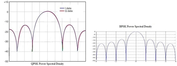
These are digital modulation techniques where in data input is digital (i.e. in binary form) and output is modulated analog spectrum as
shown below in power spectral density plot. Another input required for modulating the digital input bit stream is also analog RF carrier.
BPSK and QPSK modulations techniques have their own advantages and disadvantages and hence are used in the same wireless system for
different purpose. On this page we will compare both BPSK vs QPSK modulations and also will go through difference between BPSK and QPSK in
terms of many useful factors such as constellation diagram, robustness, power spectral density(PSD) etc.
BPSK
The short form of Binary Phase Shift Keying is referred as BPSK.
For step by step description of how bit streams get converted to BPSK symbols, refer BPSK modulation.
| Input | Output |
|---|---|
| 1 | 1 |
| 0 (0 degree) | -1 (180 degree w.r.t. reference) |
QPSK
The short form of Quadrature Phase Shift Keying is referred as QPSK.
For step by step description of how bit streams get converted to QPSK symbols, refer QPSK modulation.
| Input1 | Input2 | Output |
|---|---|---|
| -1-1*i | ||
| 1 | -1+1*i | |
| 1 | 1-1*i | |
| 1 | 1 | 1+1*i |
Usually above complex values are multiplied with 1/sqrt(2) or 0.7071 in order to normalize the modulated waveform.
After understandig the modulation types individually, now let us examine the difference between BPSK and QPSK.
As mentioned above in the table, BPSK represents binary input 1 and 0 w.r.t. change in carrier phase by 180 degree.
While QPSK represents two bits using complex carrier symbol each having 90 degree shift with one another.
BPSK is considered to be robust modulation scheme compare to the QPSK as it is easy in the receiver to receiver the original bits.
After passing both BPSK and QPSK through channel and noise, in the BPSK demodulator only two decision points are required to retrieve the original
binary information. In QPSK demodulator four decision points are needed.
With BPSK, higher distance coverage can be achieved from the base station cellular cell or fixed station
to the mobile subscribers compare to QPSK.
 BPSK vs QPSK
QPSK has advantages of having double data rate compare to BPSK.
This is due to support of two bits per carrier in QPSK compare to one bit per carrier in the case of BPSK.
Figure-2 mention difference between power spectral density of BPSK and QPSK modulated spectrum.
To take advantage of both the modulation schemes advance wireless systems such as WLAN, WiMAX, LTE utilize both for different channel or synchronization signals.
For example BPSK is used for preamble or pilot sequences or beacon frame used for channel and other synchronization purpose.
While QPSK is used for data transmission to provide higher data rate.
BPSK QPSK and other Modulation types links
Other than BPSK vs QPSK one can also refer following links which mentions difference between AM vs FM vs PM, ASK vs FSK vs PSK, about modulation basics and modulation types viz.
BPSK, QPSK, QAM, 8PSK, DPSK, MSK, GMSK, C4FM vs CQPSK etc. AM vs FM vs PM
ASK vs FSK vs PSK
what is modulation
MSK and GMSK modulation
8-PSK modulation
QPSK modulation
BPSK modulation
QAM modulation
DPSK Modulation
C4FM vs CQPSK
What is difference between
C4FM vs CQPSK
Refer QPSK vs OQPSK vs pi/4QPSK for difference between QPSK, OQPSK and pi/4QPSK modulation typesdifference between OFDM and OFDMA Difference between SC-FDMA and OFDM Difference between SISO and MIMO Difference between TDD and FDD FDMA vs TDMA vs CDMAFDM vs TDMCDMA vs GSM
Translate this page
ARTICLES
T & M section
TERMINOLOGIES
Tutorials
Jobs & Careers
VENDORS
IoT
Online calculators
source codes
APP. NOTES
T & M World Website
LMS-DD Equalizer[edit]
This equalizer is great for signals that don’t fit the constant modulus requirement of the CMA algorithm, so it can work with things like QAM-type modulations. On the other hand, if the SNR is bad enough, the decisions being made are incorrect, which can ruin the receiver’s performance. The block is also more computationally complex in its performance. When the signal is of good quality, though, this equalizer can produce better quality signals because it has direct knowledge of the signal. A common model is to use a blind equalizer for initial acquisition to get the signal good enough for a directed equalizer to take over. We won’t try and do something like that here, though.
As a challenge, take the mpsk_stage4.grc file and replace the CMA equalizer recovery with the LMS-DD equalizer and see if you can get it to converge. This block uses a Constellation Object, so part of the difficulty here is creating the proper constellation object for the QPSK signal and applying that.